Why do we need to predict physical behavior? Let’s say you want to build a boat. Turns out, it’s much cheaper to validate your boat design before you actually build the boat. To do that, you should check how your invention behaves in the destination environment before the actual manufacturing. You can do that using computer simulations which approximate the physical interactions between the water and your boat.

For a more trivial example, we can look at video games. The game below, Sea Of Thieves, is known to have one of the most realistic representations of water in the whole game industry. In this case, the simulation can be less accurate at the expense of performance since you would want the game to run as fast and smoothly as possible.

Before we continue, here is a small disclaimer: This post is a transcript of the presentation I gave during the symposium at the University of Groningen. The associated thesis will be linked here very soon. I hope, that this post provides a brief introduction to Graph Network-based Simulators and shows how I have extended this method so that it can infer the trajectory of any system based on a short video.

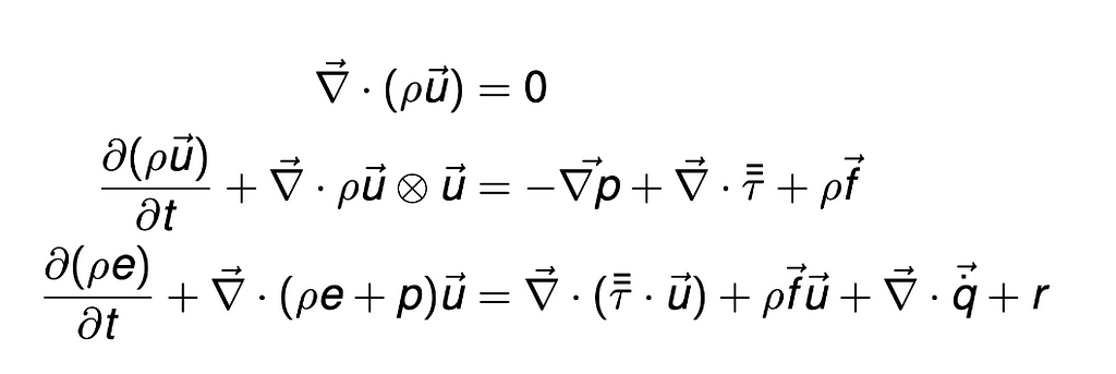
So, how do you do that? These are the Navier-Stokes Equations. They describe the motion of viscous fluid substances and can be used to describe the water flow in a pipe or an air flow around a wing of a plane. If you happen to accidentally find the solutions to them in three dimensions, hit me up, because there’s a million dollars prize if you do. So in short, math is hard. Fortunately, there are ways to approximate fluid motion without calculating this monster.

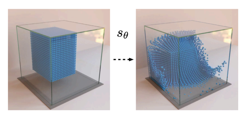
And these simulations are fast. What you see here is a simulation method called Smoothed Particle Hydrodynamics. Particles affect the other particles nearby. Describing these local behaviors and deploying them on thousands of particles can yield very accurate results. Let’s try to figure out how to build a neural network that predicts this behavior.

To do so, we need to frame the problem more explicitly. The input is a set of particles. Then, this state should pass through some funny function to come up with new positions of these particles. Repeat this process million times and we have a full simulation. Pretty easy.

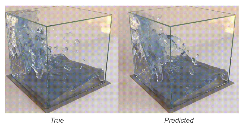
Guys at DeepMind would fully agree with that. They came up with a method that can predict the behavior of complex physical systems. One of the videos you see is the predicted trajectory, while the other one was simulated using traditional methods. Can you guess what is what?

Well, as you can see, people at DeepMind kind of know what they are doing.

Ok, but what if you want to predict the motion of sand? Then, you need to retrain a new model from scratch on a new dataset.

What if you wanna have a model that’s specialized in goop? Then again, new dataset, new training, new model.

What about something in between? What about a model that predicts goop-o-sand behavior? Again, it needs to be trained from scratch. Even if you already have a model of sand and a model of goop!

That brings us to our research question: does a video of a physical system contain enough information to generalize Graph Networks?

We want to build a system that based on a single video, can predict the behavior of the system visible in the video. Ideally, the whole system would require only a single training procedure and it would be able to generalize well across different systems.

So here’s my suggestion. We are going to build a model. This model is going to watch a video of a physical system and predict its properties in some latent space. This would allow to encode the physical properties of any system while preserving any differences between them. As you can see, the goop-o-sand lies somewhere in between sand and goop indicating that its behavior should be an “average” of these two.

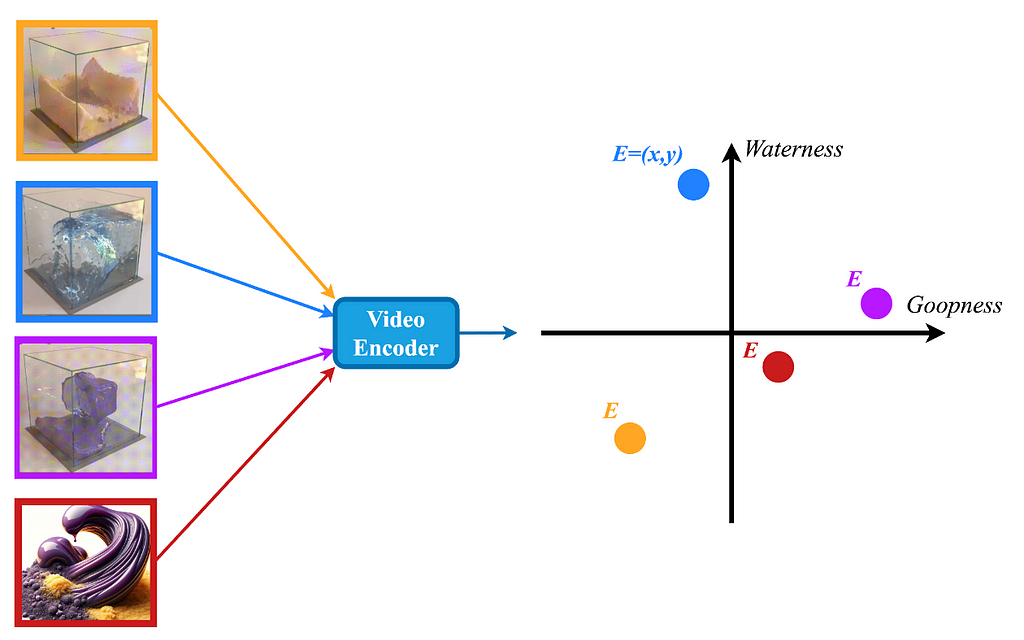
So let’s use this physical encoding to predict the system’s motion. Firstly, the Video Encoder watches a video and calculates the physical properties of the system. This encoding is going to differ based on the video that the it watched.

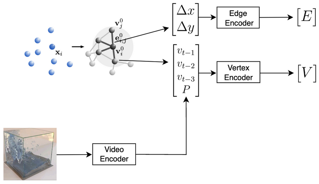
Then, this encoding is combined with the information from the original particles.

Firstly, we create a graph out of the original particles. Each particle becomes a graph vertex. The edges are created between the neighbouring particles. Each edge contains information about the displacement between the particles it connects. Each particles stores its last three velocities as well as the physical properties provided by the Video Encoder.

Now, both edges and vertices store vectors. We can pass these vectors through their respective encoders to obtain a latent graph. The encoded graph has exactly the same structure as the original one, but the encodings of edges and vertices have been updated using these small neural networks.

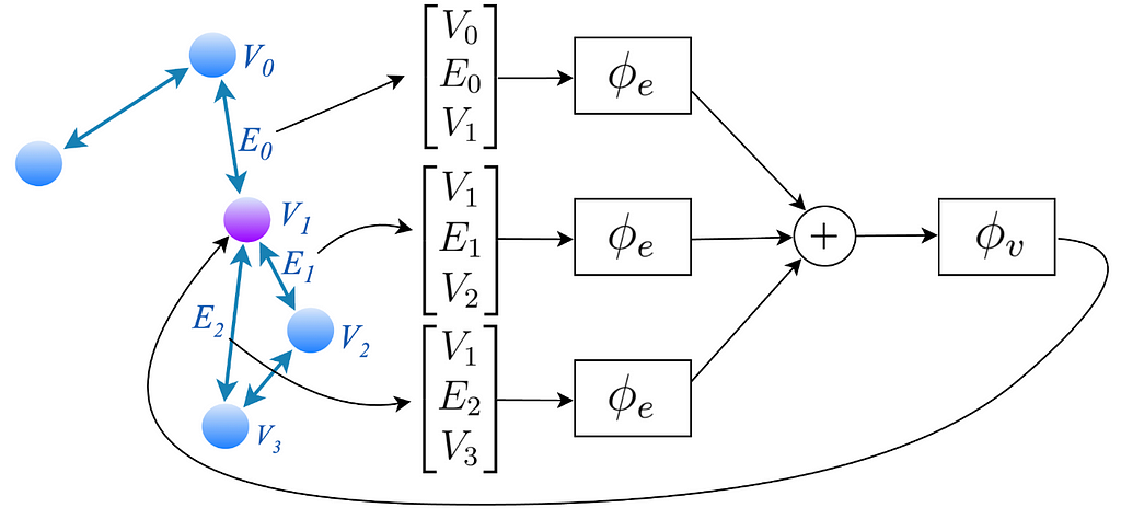
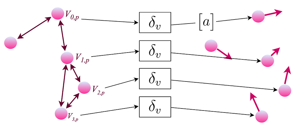
Perfect! Now, every edge has some encoding and every vertex has some other encoding. We are going to perform a procedure called message passing. In this example, we are going to focus on the purple node.

First, we find the three edges that are connected to the purple node. Let’s focus on the edge that has the E-Zero encoding. We’re going to construct a vector in the following way. Since every edge always connects exactly two nodes, we are going to take the encodings of these two nodes. In this case, V-0 and V-1. Additionally, we are also going to include the encoding of the edge itself. We repeat this procedure for every edge connected to the purple node.

These vectors are then passed through yet another neural network and then summed together.

This output finally goes through one more small module in order to obtain new node encodings. The output of this procedure is fed back into the original node. This whole procedure is then repeated again and again. In my experiments, I performed three of these message-passing steps.

Perfect! Now the last step. Each particle has an associated vector with its encoding.

We can finally decode the graph to finally obtain the acceleration of each individual particle. Since we have the acceleration, we can calculate the new velocity. With the new velocity, we can calculate the new positions for each individual particle. Now, we can repeat this whole procedure to get the state of the system at the next timestep.

Let’s test it out. Before jumping into fluids, I tested the approach I just described on a simpler system. The system consists of 10 particles, connected with springs. This setup is naturally converted into a graph where the springs are simply replaced with edges. Also, since the systems differ only in one value k, which is the spring constant, the physical encoding calculated from the video contains only a single number.

To train the model, I generated trajectories for systems with varying spring constants. On the right, you can see 5 different classes of systems. During my experiments, I varied the amount of system classes. Some models are trained only using trajectories with either very low or very high spring constants, while some are trained with even 10 distinct system classes.

In total, every dataset always contains 320 trajectories. Each trajectory is 3 seconds long, totaling 300 timesteps. Further, each sample with the graph has an associated video of the trajectory.

During the training, samples are chosen in a non-standard manner to increase the variance in the dataset. Firstly, a single timestep is chosen. This contains the input graph as well as the target accelerations. Let’s say this timestep is from a class where the spring constant k is equal to 4000. Then, out of all the videos of systems with that particular spring constant, a random one is chosen. This video is then passed to the network together with the graph in order to calculate the accelerations.

What’s important is that the video encoder is trained together with the graph network at the same time. This means that the video encoder is learning the physical properties solely based on the predicted accelerations.

And here are the results! Based on the video, the physical encoding is different. On top, you can see a video of a system with a low spring constant and its low physical encoding. On the bottom is a video of a system with stiffer springs, resulting in a high physical encoding.

On the right are the predicted trajectories. What’s interesting is that both of them started with the exact same initial condition. However, based on the physical encoding, my model managed to generate rollouts that resemble the system visible on the video. Springs in the top-right are much more flexible than the ones in the bottom-right. Before calling it a success, let’s look at some more data

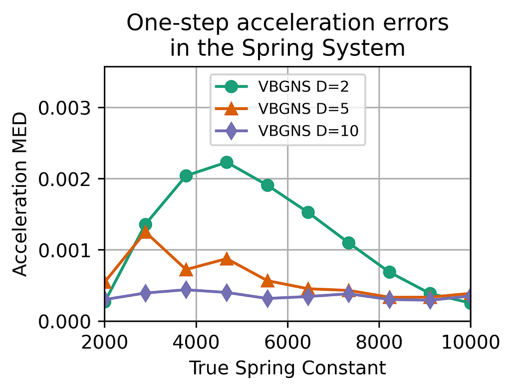
Firstly, the model that was trained using only the trajectories of two systems, either with a very low spring constant or a very high spring constant. While the one-step errors for these two classes are very low, the errors are way larger for the systems that are somewhat in between. That’s likely because the model has only seen those extreme cases, hence it cannot interpolate that easily between them.

If the model is trained with 5 different classes, a similar phenomenon occurs, the errors are low for the systems present during training and higher for the ones that the model has never seen.

Finally, the errors are the lowest if the model has seen 10 different systems with 10 different spring constants. These results align with the intuition of neural networks since they do a very good job when dealing with data present in the original distribution but have trouble going out of distribution.

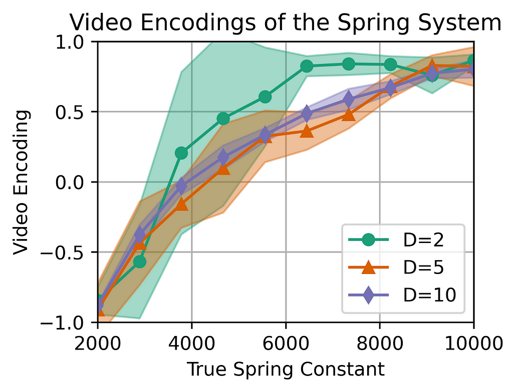
Another interesting thing I wanna show you are the physical encodings. In the first model, the mean encoding of various systems seems to clearly correspond to the true spring constant.

Similar things can be said about the other models. There is also a clear correspondence between the true spring constant the the predicted video encoding.

What’s interesting now, is the variance of these encodings. The highlighted region represents the standard deviation of the results. As you can see, the variance is low for the systems that are present in the original distribution and is quite large for the systems that were not present in the training dataset.

For the model trained with 5 classes, the variance is visibly smaller indicating that the model is more “confident” in its predictions.

This effect is even larger for the final model trained on 10 system classes.

Based on what we know let’s answer the original question. Can we use a short video to reliably encode physical properties of the system?

Yes, we can. Can we train the whole system in one single procedure?

Yes, we can. Finally, can we reliably interpolate between different materials?

Kind of, as we have seen, models struggle generalizing outside of the distribution. However, as the training distribution becomes more granular and contains more variation in the system classes, the errors become way smaller across the spectrum.

Thank you for reading through this blog post. It would mean a lot if you let me know what you think about my work! Cheerios :)